Unsupervised learning - Dimensionality reduction and clustering
Unsupervised learning forms an important part of Machine learning. On unlabeled data, the main task is to find uncovering hidden patterns, structures, or groupings.
What are the unsupervised learning tasks?
1. Density Estimation
Estimate the underlying probability distribution of the data.
Examples:
-
KDE,GMM - Applications: anomaly detection, generative modeling
2. Clustering
Group similar data points based on feature similarity.
Examples:
-
KMeans,DBSCAN,Agglomerative Clustering - Applications: customer segmentation, image grouping
3. Dimensionality Reduction
Reduce the number of input features while preserving important structure in the data.
Examples:
-
PCA,t-SNE,UMAP - Applications: data visualization, feature extraction
1. Density estimation
Parametric methods - Assume the data follows a known distribution form (e.g. Gaussian) and fit parameters.
- Gaussian Mixture Models (GMMs): A flexible model that represents the data as a mixture of multiple Gaussians. Each component has its own mean and covariance, allowing the model to approximate complex shapes. GMMs assume that the data is generated from a mixture of several Gaussian distributions, which may not always be the case in real-world scenarios.
Non-parametric methods - Make fewer assumptions about the data distribution.
- Kernel Density Estimation (KDE): KDE places a kernel (e.g. a Gaussian bump) at each data point and sums them to get a smooth estimate of the density function. The bandwidth (smoothing parameter) controls how spiky or smooth the estimate is.
2. Clustering: algorithm and evaluation
Evaluation of clustering
Unlike supervised learning, we don’t have true labels. Evaluation metrics include:
- Internal: Silhouette score, Davies-Bouldin index
- External (when ground truth exists): Adjusted Rand Index, Mutual Information
Why DBSCAN is so powerful?
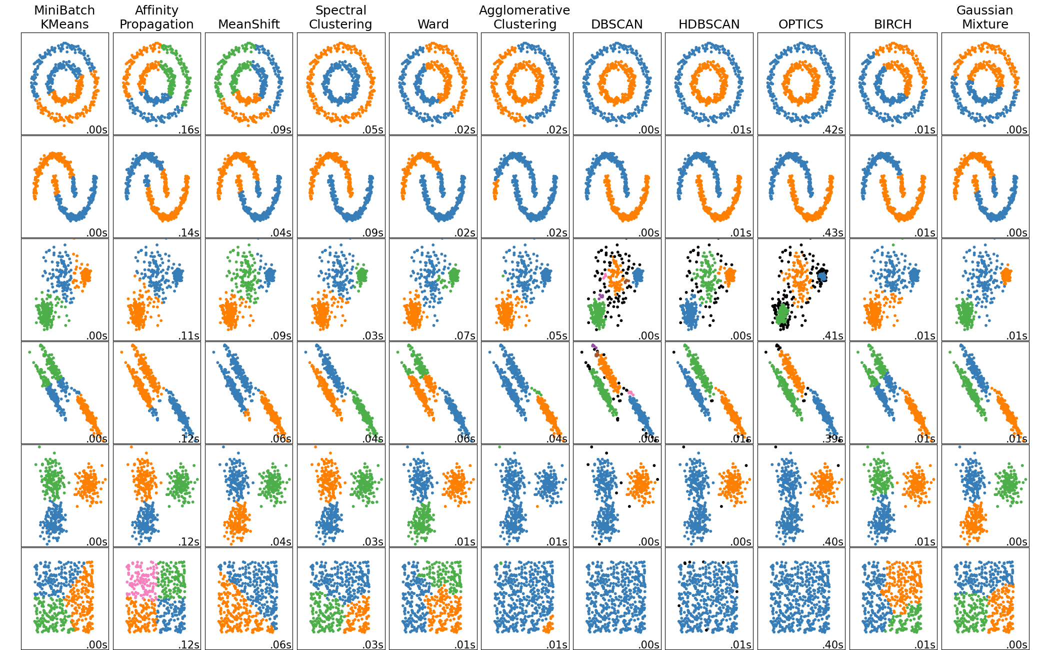
(Scikit-learn documentation shows a comparison of different clustering methods.)
DBSCAN (Density-Based Spatial Clustering of Applications with Noise):
- Can find arbitrarily shaped clusters
- Automatically detects outliers as noise
- Does not require the number of clusters to be specified in advance
- Especially useful in real-world noisy data with non-spherical structures
3. Dimensionality reduction: Are they real clusters?
Dimensionality reduction techniques like PCA, t-SNE, and UMAP are widely used to project high-dimensional data into 2D or 3D space for visualization. These methods can help uncover apparent clusters or structures. However, it’s important to remember that not all visual clusters represent true separations or clustering in the original space.
PCA
Principal Component Analysis (PCA) is a linear dimensionality reduction technique that projects the data onto the directions of maximum variance. It assumes that the most informative structure in the data can be captured through orthogonal linear combinations of the input features.
PCA is closely related to Singular Value Decomposition (SVD) in linear algebra.
t-SNE and UMAP
When linear projections like PCA are not enough to separate complex patterns, nonlinear techniques like t-SNE and UMAP come into play.
- t-SNE (t-distributed Stochastic Neighbor Embedding):
- Focuses on preserving local structure
- Uses pairwise similarities and minimizes KL divergence
- Often produces visually compelling clusters, but does not preserve global distances
- UMAP (Uniform Manifold Approximation and Projection):
- Based on manifold learning and algebraic topology
- Preserves more global structure than t-SNE
- Faster and more scalable
- Generalizes well to new data
A deeper dive into the UMAP method
UMAP combines manifold learning, algebraic topology, and optimization into a powerful visualization tool.
UMAP is built on a few key mathematical ideas:
-
Manifold Assumption
Assumes data lies on a low-dimensional manifold embedded in high-dimensional space. -
Fuzzy Topological Representation
Constructs a fuzzy simplicial set (probabilistic k-NN graph) to represent high-dimensional relationships. -
Cross-Entropy Optimization
Learns a low-dimensional embedding by minimizing the cross-entropy between high- and low-dimensional graphs.
User comment
While we know that UMAP has some randomness controlled by the random seeds, I find out that points that are exactly the same in the high dimensional space of a batch may appear to be different in the low dimensional representaion space. This is because the inherent stochasticity and numerical issues of the UMAP calculation.
Reference
[1] McInnes, Leland, John Healy, and James Melville. “Umap: Uniform manifold approximation and projection for dimension reduction.” arXiv preprint arXiv:1802.03426 (2018).